Introduction to R
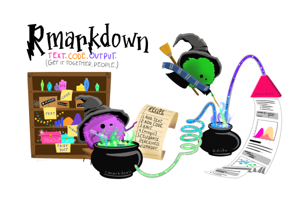
 all artwork by @allison_horst
My Experiences Teaching R
Installing R and RStudio
-
R is a free, open source programming language that is often used for statistical and data analyses and visualizations
-
RStudio is an IDE (integrated development environment) for R
-
You will need to install/download both R and RStudio
-
You can install R from the CRAN (Comprehensive R Archive Network) website. I suggest downloading the latest version, which (as of the time of writing this blog) is R 4.1.1
-
You can download RStudio here
-
Although you need to have R installed, you will mostly likely never need to open R because you can do everything you need in RStudio
Getting familiar with RStudio
There are 4 panes you will quickly become very familiar with within RStudio
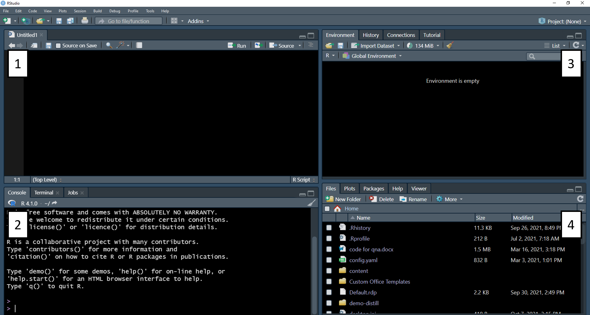
- Top Left: This is the Source Editor where you write scripts
- To test it out, you can go File → New File → R Script
- Bottom Left: This is the Console where you can type code that you want to run one time and don’t want to save it to a script. If you run a line of code in a script, depending on your settings, you may see the output in your console
- Top Right: There are quite a few tabs here, but the most important tab for beginners is the Environment tab where you can see all of your saved variables and objects
- Bottom Right: There are also several tabs here, but here you can see:
- Files that are located within your working directory
- Your beautiful plots and visualizations
- Packages that you already have or would like to install
- Help documentation. This is a really great built in feature to help you understand specific functions. To test this out type
?meaninto the console and you will see the documentation for the mean() function. This is incredibly useful to see what the function looks like, including what arguments it takes, and often there will be examples at the bottom of the documentation with code for you to test out the function.
Working Directory
Before getting started with some coding, it’s important to understand what a working directory is.
- What is a working directory? A working directory (wd) is the location where R will look for files. This is where R believes you are located.
- How do you know what your wd is? In the console type
getwd()to see what’s called your “current working directory”. You may notice that this path will most likely align with the path at the top of the Files tab because, again, this is where R thinks you are located. If you want load in any files, you must be in the correct working directory or R will return an error sayingcannot open file x: No such file or directory - How do you set your wd? There are a few ways you can do this…
- Option 1 (not recommended): Session → Set Working Directory → Choose Directory and navigate to find the correct folder
- Option 2 (also not recommended):
setwd()to manually enter the path you want - Option 3 (highly recommended!): Create an R Project that will automatically set your wd to where your project is saved
R Projects
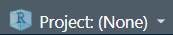
- What is an R Project? An R project is just a way to keep all of your files associated with any given project together, organized, and easily accessible. If you wish to test out how to set up an R Project, following along with the next few steps. Take a look in the top right hand corner of RStudio and you will see a blue R cube. Assuming you haven’t already created a project, it will say “Project: (None)”. To create a new project, click on that and select New Project. You will see the following options:
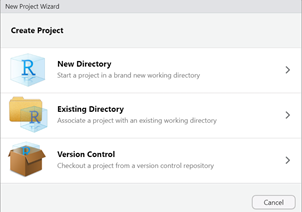
This is where you decide where you want your project to be located. If you already have an existing folder choose “Existing Directory” and navigate to the correct folder and create your project. If you want to create a new folder choose the “New Directory” and New Project. Here you will have to create a name for your directory and again select where you want your project to be located and then Create Project. We won’t worry about the version control option for now, but you may find it super handy, especially if you use GitHub.
Once you’ve created your project, I suggest closing out of RStudio and navigating to your files where you just saved your project. You should see the familiar looking R cube with your directory name. Now all you have to do to open your project is double click on this R cube. RStudio will automatically open and you can type getwd() in the console to confirm you’re in the correct location and you files will be in the Files tab. If you followed along with these steps, congrats on setting up your first R project! 😄
R Scripts
Now that we’ve covered some of the basics, let’s write our first R script!
To start, click File → New File → R Script. Let’s first save our script by clicking on the save icon or ctrl/cmd + S. As I’m not very creative… I’ll call my script “r_script”.
I recommend saving this in the same location as your R Project so it’s all in the same place and easy to find. If you click on the Files tab, you should see your script is now there! For me, I now have a file called r_script.R - notice it has automatically added the extension .R as it’s an R Script. You can also see it says R Script in the bottom right corner of your Source Editor.
Great, let’s start coding!
# type or copy the following code into your script:
print("My first script!!")

10 + 20 + 30

x = 1 + 2 + 3
Okay a few things to go over here:
- Anything written after a # is “commented out”. This means R won’t read or evaluate anything following a #. This is perfect for leaving comments or notes to yourself like I have done above
- To run your entire script, click Source and then Source with echo (echo will print out your code along with the output)
- You should see that the first line of code printed “My first script!!”
- The second line of code printed the output “60”
- But, the last line of code didn’t print any output. This is because the last line we are defining a variable “x”. So, although nothing is printed in our console output, check out your Environment - you should see you now have your variable “x” saved there and it’s value is 6!
- Because you have x saved in your environment, now if you type x in your console, you will see the output
- You can also run your script line by line. One way to do this is put your cursor on the line you want to run and click the green Run button. Or, put your cursor on the line you want to run and press ctr (or cmd) + enter. You’ll see your cursor moves down a line automatically after you run one line. So if you start at the top of your script and press and hold down ctrl and press enter 3 times, all 3 lines of code will run.
R Markdown
When I started coding, I only used R scripts. But then I discovered R Markdown and now I use .Rmd scripts exclusively. R Markdown is a great way to create beautiful reports with a mix of text/notes and code. R Markdown files can also be easily converted to html, pdf, or word docs.
So, now let’s create our first Rmarkdown script!
Click File → New File → R Markdown.. and enter a title for your script - I’ll title mine “My Rmarkdown Script” (note: the title here can have spaces). I’ll stick with the default HTML format, so then can click Okay. Notice now that the bottom right hand corner of the source editor now says R Markdown. Even though we created our file and provided a title, we still have to save our file. I’ll save mine as rmd_script and the .Rmd extension will again be added automatically.
When we created our .R script, we had a blank script, but now we see that we are provided with a default template. There are 4 things I want to quickly point out here, but will go into more detail of each below.
- The YAML header section: this is located at the top of our markdown file, enclosed by
--- - R chunks: if you want to write code, you have to create an R chunk, which will always have this formatting: ```{r }…```. This is an example of one:

-
All other space: everything outside of the YAML and R chunks is for writing text. Remember, R Markdown is a meant for integrating content/text along with code. So, everything here will be text written in the markdown language and there’s no need for the # like we needed in our R script.
-
You may have noticed in our .Rmd script (at the top) we have a new
Knitbutton that we didn’t have in our .R script. Go ahead and press this button to watch R knit your file from R to html (because that’s what we’ve specified the output to be). Your “knitted” file will either appear in the Viewer pane or in a new window depending on your settings. Here we see we have our title, some text, some code, and even a plot! Pretty cool right?!
Now, let's spend a little more time discussing each of these sections in more detail.
YAML Section
In our default YAML, we already have a title and output specified. There are other arguments you can add here, such as author or date. Let’s add the author argument to test it out.
Try knitting your file again. Now you should see your name appear under the title.
---
title: "My Rmarkdown Script"
output: html_document
author: Jenny Sloane
---
author:Jenny Sloane without the space I would have issues with knitting my document.
R Chunks
We already have a few chunks created for us in our template. In any code chunk, you’ll see a few buttons in the top right corner: an options/gear button and 2 arrows.
- The gear button allows you to modify chunk options (I don’t think I’ve ever used this).
- Next to the gear button, there’s an arrow pointing down, which if you click it will run all of the chunks above the current chunk.
- Finally, the green arrow pointing to the right will run all of the code within that current chunk. Of course you can also run your code line by line the same way as we did in the .R scripts (I usually navigate to the chunk I want to work on, press the arrow pointing down, and then run my code line by line by pressing ctrl + enter).
R chunks have certain options you can set. For example, if you want the actual code to appear in your knitted document, you can set echo=TRUE and if you only want the output to appear and no code you can set echo=FALSE. Other chunk options that I often use are: include, warning, message, and eval.
The first chunk you see in the template is a little bit different. While this chunk is not necessary and you can remove it if you’d like, this is where you can set global chunk options. For example, you can see echo is set to TRUE here, so this means all of the code will appear in your knitted document. You can override the global chunk settings by directly adjusting the options in any specific chunk.
As a small aside, you may have noticed next to the r in the example chunk above it says “pressure”. This is where you can set a “name” for you chunk, so it makes sense that this chunk is called pressure as it’s plotting pressure. This is just another way to help keep your code and report organized.
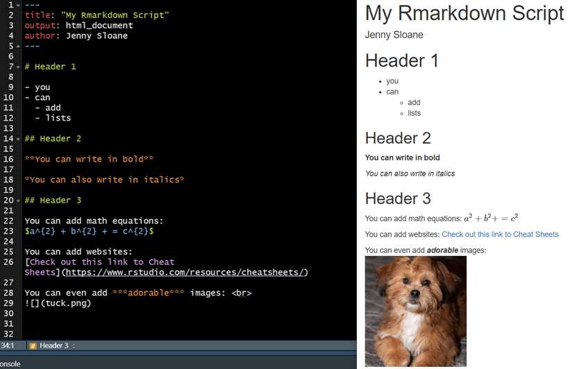
Markdown
All text outside of the YAML and R chunks is written with Markdown syntax. You can easily style your text with bold and italics. You can add headers, lists, equations, links, images, and so much more. Below you can see what code looks like in R Markdown compared to what it looks like when it’s knitted to a pdf.
Tidyverse!!
I first learned R in base R, but once I learned about tidyverse there was no going back. There’s so much I can say about tidyverse, but I’ll only cover some of the basics and continue to provide resources along the way.
What is tidyverse?
Tidyverse is a collection of 8 packages (ggplot2, dplyr, tidyr, readr, purrr, tibble, stringr, forcats) introduced by Hadley Wickham to help with data manipulation, exploration, and visualisation.
- Check out the tidyverse website to find out more details of each of the individual packages
Installing tidyverse
Whenever you want to use a package, the first thing you have to do is install the package. Once you install a package, it will remain installed on your computer, so you only have to install it once (I always install packages in my console as there’s no need to save it to a script)
- The code to install tidyverse looks like this
install.packages("tidyverse") - The install.packages() functions will install packages that are part of CRAN (Comprehensive R Archive Network)
Installing non-CRAN packages
- However, not all packages are part of CRAN (especially one’s that are still in development). If you get a warning like the
package ‘xxx’ is not available for this version of R, that’s a good indication that it’s not on CRAN. - If it’s not on CRAN, you’ll need to locate the repository on GitHub and install via
devtools.- For example, if I wanted to install the package “emo” for emojis 🎉 , I would type in something like “emo package R” into Google and search for the GitHub page, which would be https://github.com/hadley/emo. There are instructions for how to install the package in the ReadMe document if you scroll down on the page.
Loading tidyverse
It’s not enough to just install the package. Every time you start a new R session, you need to load in the packages you wish to use, so I always put this code within my script as it needs to run every session.
- The code to load the package looks like this:
library(tidyverse) - Whenever you load tidyverse, you will see a message saying it’s attaching all 8 packages. Therefore, you don’t have to load in any of the individual packages because they all get called in together. This means as long as you load in tidyverse, you can use functions from any one of the 8 packages.
So, you can think about it as having an entire library of all the packages you’ve ever installed. But, in each script and session you need to specify which libraries (aka packages) you want to load in.
The Pipe %>%
This is the pipe operator: %>%
If you use tidyverse, you will quickly become very familiar with this operator. You use the pipe when you want to execute multiple operations in a specific sequence. To me, it makes sense to think about the pipe as “AND THEN”.
For example:
I want to do x AND THEN
I want to do y AND THEN
I want to do z
which is equivalent to:
I want to do x %>%
I want to do y %>%
I want to do z
For a real example, let’s look at some code below. In the code, we’ll first load in tidyverse and the palmerpenguins libraries (you may need to install it if you’ve never used it before). With the palmerpenguins package, there’s a built in penguins dataset that we’ll explore.
library(tidyverse)
library(palmerpenguins)

head(penguins) # gives us the first 6 rows of our dataset
## # A tibble: 6 x 8
##   species island bill_length_mm bill_depth_mm flipper_length_~ body_mass_g sex
##   <fct>   <fct>           <dbl>         <dbl>            <int>       <int> <fct>
## 1 Adelie  Torge~           39.1          18.7              181        3750 male
## 2 Adelie  Torge~           39.5          17.4              186        3800 fema~
## 3 Adelie  Torge~           40.3          18                195        3250 fema~
## 4 Adelie  Torge~           NA            NA                 NA          NA <NA>
## 5 Adelie  Torge~           36.7          19.3              193        3450 fema~
## 6 Adelie  Torge~           39.3          20.6              190        3650 male
## # ... with 1 more variable: year <int>
levels(penguins$island)
## [1] "Biscoe" "Dream" "Torgersen"
levels(penguins$species)
## [1] "Adelie" "Chinstrap" "Gentoo"
From quickly looking at the levels of a couple of variables, we can see there are 3 islands (Biscoe, Dream, Torgersen) and 3 species (Adelie, Chinstrap, Gentoo).
I like the idea of a “Dream” island, so the question I’ll ask here is:
Here’s the code to answer my question and below I’ll go through the pipes line by line:
penguins %>%
  select(species, island, body_mass_g, sex) %>% # step 1
  filter(species == "Adelie" & island == "Dream") %>% # step 2
  group_by(sex) %>% # step 3
  summarise(mean_body_mass = mean(body_mass_g)) %>% # step 4
  drop_na() # step 5
## # A tibble: 2 x 2
##   sex    mean_body_mass
##   <fct>           <dbl>
## 1 female          3344.
## 2 male            4046.
- Step 1: First, from the penguins data, I’m selecting only the variables I’m interested in AND THEN…
- Step 2: I’m filtering my data to only have the Adelie species and only from Dream island AND THEN…
- Step 3: I’m grouping by sex in order to get an average body mass calculation for males and females AND THEN…
- Step 4: I’m summarizing my data to get the mean body mass AND THEN…
- Step 5: I’m dropping the NA values
And finally, we see our output: the mean body mass for females Adelie penguins on Dream island is 3344 grams and 4046 grams for males
dplyr functions I use all the time (i.e. select(), filter(), group_by(), summarise(), and drop_na()).
My Workflow
In this final section, I thought I’d share some tips and an example of my workflow in R. There are many free datasets you can explore within R (e.g. mtcars, iris, penguins from the palmerpenguin package). However, for this blog, I’ve downloaded a dataset from Kaggle on the medal standings from the Tokyo Olympics.
Usually when I use R, I have a folder within the root of my project titled “data” and of course this is where I keep the actual data files. This just helps me keep my project more organized and I always know exactly where my data is. So, I’ve done the same thing here - I created a data folder and saved my medals.csv file there. Note, that this is now one folder “deep” into our project. What this means is that we have to let R know to look inside the “data” folder in order to find our .csv file because it’s not located at the root of our project. But don’t worry, this is easy to do, especially if you know about the here package.
Below I’ll show you my typical workflow using the medals dataset.
Load in libraries
library(tidyverse)
library(janitor)
library(here)
library(ggeasy) # this is an awesome package to help customize ggplots with easy to remember functions
- My first chunk of code is always dedicated to loading in all of the libraries I need for my entire script
- I make sure the chunk options include
message=FALSEandwarning=FALSE, so when I knit the file I don’t see all of the messages and warnings from loading in the respective libraries
Read in data
medals_raw <- read_csv("data/medals.csv")
# medals_raw <- read_csv(here("data", "medals.csv")) # this will also work, if you wish to use the here package

head(medals_raw) # look at only the top 6 rows
## # A tibble: 6 x 7
##    Rank `Team/NOC`                  Gold Silver Bronze Total `Rank by Total`
##   <dbl> <chr>                      <dbl>  <dbl>  <dbl> <dbl>           <dbl>
## 1     1 United States of America      39     41     33   113               1
## 2     2 People's Republic of China    38     32     18    88               2
## 3     3 Japan                         27     14     17    58               5
## 4     4 Great Britain                 22     21     22    65               4
## 5     5 ROC                           20     28     23    71               3
## 6     6 Australia                     17      7     22    46               6
read_csv()is very similar toread.csv(), except it will automatically read your data in as a tibble (a “tidy” dataframe). For this reason, I exclusively useread_csv()- I could also use the
here()function to tell R that I want it to go within the “data” folder I just created in order to find the “medals.csv” file - We can take a look at the first 6 rows of our raw data using
head()
here package by Jenny Richmond
Clean our data
medals_top5 <- medals_raw %>% # create a new variable with our results
  clean_names() %>% # step 1
  select(team_noc, total) %>% # step 2
  arrange(desc(total)) %>% # step 3
  top_n(5) # step 4
- Step 1: When looking at the data, the first thing I notice is the variable names could be “cleaner”.
- We always want to try to avoid white space, so we’ll want to change our variable “Rank by Total”. Programmers have their own style of coding in order to avoid white space. For example, there’s “snake_case” (Rank_by_Total) or “camel case” (rankByTotal) or “kebab case” (Rank-by-Total).
- My preference is snake case and I also make sure my variables are all lowercase (mainly because, like most programmers, I’m lazy and it’s much easier to type lower case letters than capital letters)
- Fortunately,
janitor::clean_names()does all of this for me in just one line of code! - So, here I’ll use the
clean_names()function to remove white space and transform everything to lower case
- Step 2: Select only the columns/variables I need in order to answer my research question. This will make your life so much easier, especially if your dataset has dozens or even hundreds of variables
- Step 3: Arrange the total column in descending order
- Step 4: Select only the top 5 rows… I’ve actually never heard of
top_n()before, but I just did a quick Google search and found it!
And here we’re simply printing out our results:
medals_top5
## # A tibble: 5 x 2
##   team_noc                   total
##   <chr>                      <dbl>
## 1 United States of America     113
## 2 People's Republic of China    88
## 3 ROC                           71
## 4 Great Britain                 65
## 5 Japan                         58
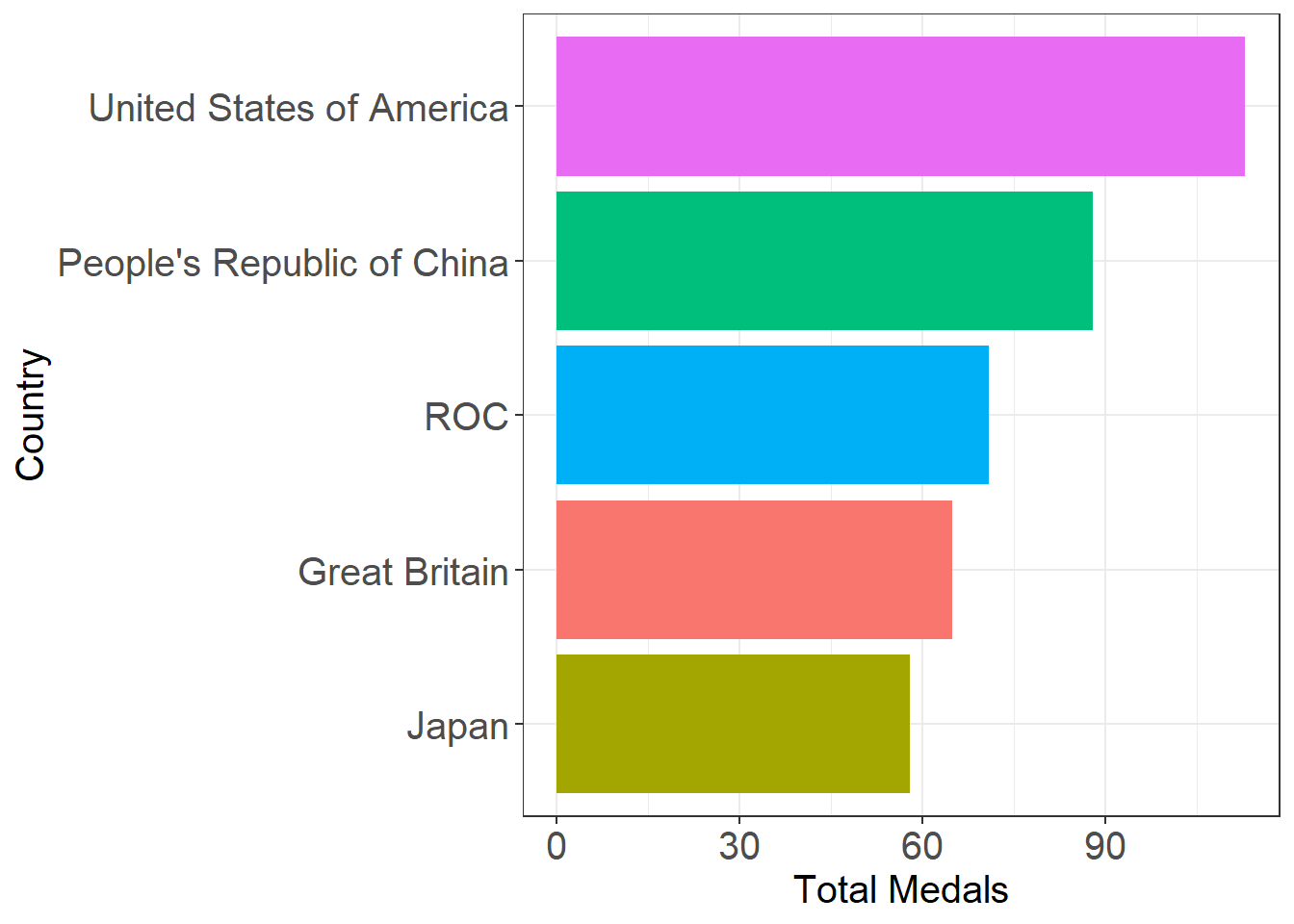
Visualise our results
Finally, let’s create a visualisation using ggplot!
- Notice that we use the
+sign rather than the%>%when using ggplot. This may get a little bit confusing at first, but this may be helpful: when using ggplot, think about it as each line is adding a new layer to your plot
ggplot(medals_top5, aes(x = reorder(team_noc, total, sum), y = total, fill=team_noc)) + # I've reordered the columns based on the sum of the total variable
  geom_col() +
  coord_flip() + # flips the cartesian coordinates to make it easier to read the country names
  labs(x = "Country", y = "Total Medals") + # you can also add a "title" here if you'd like
  theme_bw() + # there are several default themes but I like this one
  easy_remove_legend() + # one of my favorite functions from ggeasy to remove the legend
  easy_text_size(15) # another one of my favorite functions from ggeasy to change the text size
ggplot challenge
I thought it would be fun to end this blog with a bit of a challenge for you to test out all of your new R skills! I’ve included a few hints below, but remember Google is your best friend.
Thanks so much for reading this blog and feel free to share your plots on Twitter and tag me @jfsloane - I’d love to see!
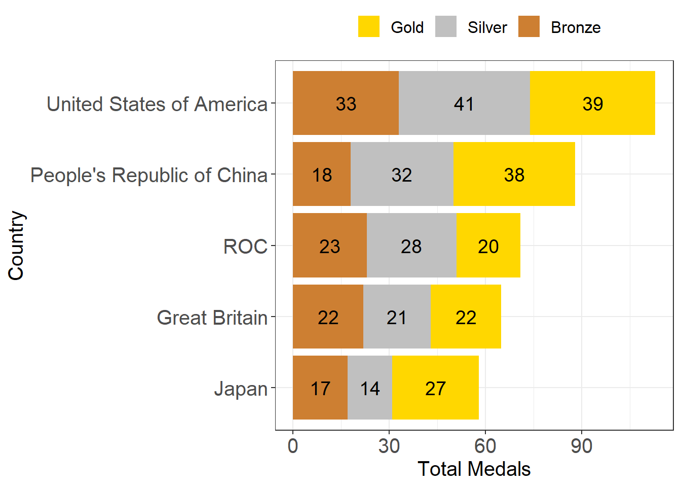
- I’ve used the 5 countries with the most total medals (the same countries as I plotted in the graph above in the section on “Visualise our results”)
- The medal types (gold, silver, bronze) are in a “wide” data format. In other words, gold, silver, and bronze all have their own columns. However, ggplot likes data in a “long” format, so this is the perfect time to look up and learn about
pivot_longer() - The type of graph I’ve plotted is called a “stacked barplot”
- I’ve manually set the colors using hex codes to get gold =
#FFD700 , silver =#C0C0C0 , and bronze =#CD7F32
Jennifer Sloane
Quantitative Methodologist
My research interests include studying cognitive psychology, medical decision-making, coding experiments, and analyzing data